One Way ANOVA with Minitab
What is One Way ANOVA with Minitab?
The One way ANOVA with Minitab is a statistical method to compare means of two or more populations.
- Null Hypothesis(H0):
- Alternative Hypothesis(Ha): At least one μi is different, where i is any value from 1 to k
It is a generalized form of the two sample t-test since a two sample t-test compares two population means and one-way ANOVA compares k population means where k ≥ 2.
Assumptions of One Way ANOVA
- The sample data drawn from k populations are unbiased and representative.
- The data of k populations are continuous.
- The data of k populations are normally distributed.
- The variances of k populations are equal.
How ANOVA Works
ANOVA compares the means of different groups by analyzing the variances between and within groups. Let us say we are interested in comparing the means of three normally distributed populations. We randomly collected one sample for each population of our interest.
- Null Hypothesis(H0): μ1 = μ2 = μ3
- Alternative Hypothesis(Ha): One of the μ is different from the others
Based on the sample data, the means of the three populations might look different because of two variation sources.
- Variation between groups there are non-random factors leading to the variation between groups.
- Variation within groups there are random errors resulting in the variation within each individual group.
What we care about the most is the variation between groups since we are interested in whether the groups are statistically different from each other. Variation between groups is the signal we want to detect and variation within groups is the noise which corrupts the signal.
ANOVA is a modeling procedure, which means we are using a model to try to predict results. To make sure the conclusions made in ANOVA are reliable, we need to perform residuals analysis.
Good residuals:
- Have a mean of zero
- Are normally distributed
- Are independent of each other
- Have equal variance
The difference between the actual and predicted result is called a residual or unexplained variation
Run a One Way ANOVA with Minitab
Case study: We are interested in comparing the average startup costs of five kinds of business.
Data File: “One Way ANOVA” tab in “Sample Data.xlsx”
- Null Hypothesis (H0): μ1 = μ2 = μ3 = μ4 = μ5
- Alternative Hypothesis (Ha): At least one of the five means is different from others
Step 1: Test whether the data for each level are normally distributed.
- Click Stat → Basic Statistics → Graphical Summary.
- A new window named “Graphical Summary” pops up.
- Select the “Cost” as the variable.
- Click in the blank box right next to “By variables (optional)” and the “Business” appears in the list box on the left.
- Select the “Business” as the “By variables (optional).”
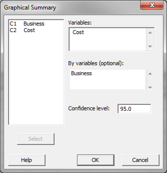
- Click “OK.”
- The normality results appear in the new window.
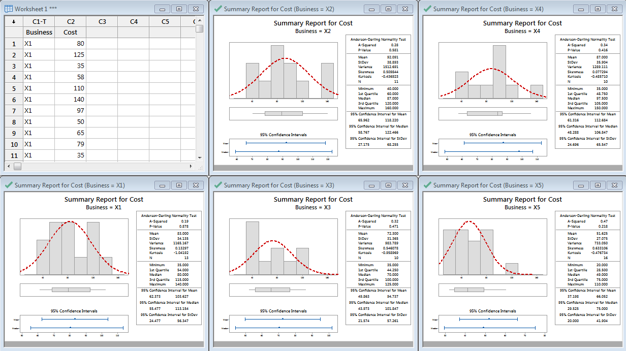
Notice all of the p-values are greater than 0.05; therefore, we fail to reject the null hypothesis that the data are normally distributed.
- Null Hypothesis(H0): The data are normally distributed.
- Alternative Hypothesis(Ha): The data are not normally distributed.
Since the p-values of normality tests for the five data sets are higher than alpha level (0.05), we fail to reject the null hypothesis and claim that the startup costs for any of the five businesses are normally distributed. If any of the five data sets are not normally distributed, we need to use other hypothesis testing methods other than one-way ANOVA. In this example, all five data sets are normally distributed; however, if any of them were not normally distributed, we would need to use another hypothesis test.
Step 2: Test whether the variance of the data for each level is equal to the variance of other levels.
- Null Hypothesis(H0):
- Alternative Hypothesis(Ha): at least one of the variances is different from others
- Click Stat → ANOVA → Test for equal variances.
- A new window named “Test for Equal Variances” pops up.
- Select the “Cost” as the “Response.”
- Select the “Business” as the “Factors.”
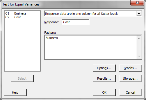
- Click “Options.”
- Select “Use test based on normal distribution”

- Click “OK” to close the “Options” window
- Click “OK” to run the test
- The results show up in a new window.
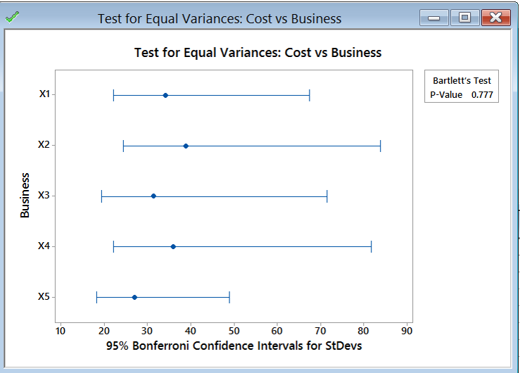
Use the Bartlett’s test for testing the equal variances between five levels in this case since there are more than two levels in the data and the data of each level are normally distributed. The p-value of Bartlett’s test is 0.777, greater than the alpha level (0.05), so we fail to reject the null hypothesis and we claim that the variances of five groups are equal. If the variances are not all equal, we need to use other hypothesis testing methods other than one-way ANOVA. If this test suggested that at least one variance was different, then we would need to use a different hypothesis test to evaluate the group means.
Step 3: Test whether the mean of the data for each level is equal to the means of other levels.
- Null Hypothesis(H0): μ1 = μ2 = μ3 = μ4 = μ5
- Alternative Hypothesis(Ha): at least one of the means is different from others
- Click Stat → ANOVA → One-way.
- A new window named “One-Way Analysis of Variance” pops up.
- Select “Cost” as “Response.”
- Select “Business” as “Factor.”
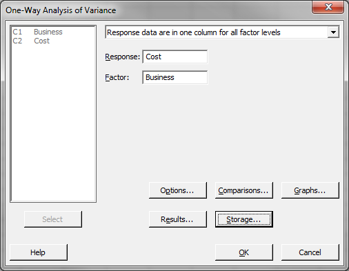
- Click “Storage.”
- Check the boxes next to “Fits” and “Residuals”

- Click “OK” to close the “Storage” window
- Click “OK.”
- The ANOVA results appear in the session window. The fitted response and the residuals are stored in the data table.
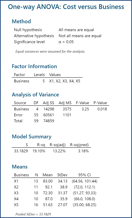
Since the p-value of the F test is 0.018, lower than the alpha level (0.05), the null hypothesis is rejected and we conclude that the at least one of the means of the five groups is different from others.
Step 4: Test whether the residuals are normally distributed with mean equal zero. The residuals have been stored in the data table in step 4.
- Click Stat → Basic Statistics → Graphical Summary.
- A new window named “Graphical Summary” appears.
- Select “RESI” as the “Variables.”
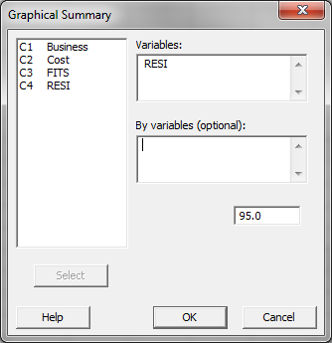
- Click “OK.”
- The normality test results show up in a new window.

The p-value of the normality test is 0.255, greater than the alpha level (0.05), and we conclude that the residuals are normally distributed. The mean of the residuals is 0.0000.
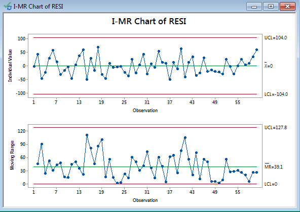
Step 5: Check whether the residuals are independent of each other. If the residuals are in time order, we can plot IR charts to check the independence. When no data points on the IR charts fail any tests, the residuals are independent of each other. If the residuals are not in time order, the IR charts cannot deliver reliable conclusion on the independence.
- Click Stat → Control Charts → Variables Charts for Individuals → I-MR.
- A new window named “Individuals – Moving RangeChart” pops up.
- Select “RESI1” as the “Variables.”
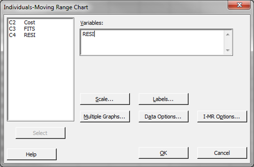
- Click “OK.”
Next, we check to determine if the residuals are independent of each other. In Minitab, we use an Individuals–Moving Range control chart (called IR here) to determine independence. If the data points are in control (not failing any of the control chart tests) we can conclude that the residuals are independent.
No tests failed; therefore, the residuals are independent.
Step 6: Plot residuals versus fitted values and check whether there is any systematic pattern.
- Click Graph → Scatter Plot.
- A new window named “Scatterplots” pops up.
- Click “OK.”
- A new window named “Scatterplot– Simple” pops up.
- Select the “RESI” as the “Y variables.”
- Select the “FITS” as “X variables.”
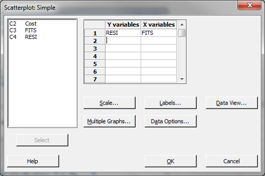
- Click “OK.”
- The charts appear in a new window.
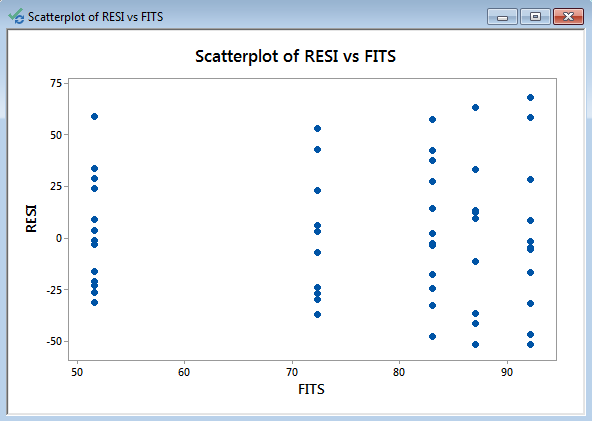
Model summary: If the data points spread out evenly at any of the five levels, we claim that the residuals have equal variances across the five levels.

